Train Your Own Encoder-Free VLM in $100

Google DeepMind latest Gemma 4 is an encoder-free multimodal model. In this blog, we’ll find out why it’s cool, and then we’ll train our own for under $100!

Classical Multimodal Models

A model that takes images, audio, and text as input and generates text as output typically consists of three transformers stitched together.

The vision encoder is usually a Vision Transformer. It takes the raw image, splits it into patches, converts each patch into a vector, and runs many attention layers over them to produce a sequence of embeddings rich with visual meaning. It was pretrained on hundreds of millions of image–text pairs, so it already “knows” a lot about the visual world. Similarly, the audio encoder turns a raw waveform into a sequence of vectors called audio embeddings, again using a stack of attention layers. After a sequence of embeddings leaves an encoder, each embedding in that sequence gets multiplied with a matrix called connector to project it to the dimension the language model expects.

Are Encoders Really Necessary?

Have you ever wondered whether the encoders are absolutely necessary? Someone at DeepMind did, and they found the answer is no. Here is one intuitive way to think about this: the encoder’s job is to turn pixels into vectors that the language model can make sense of. If the language model is powerful enough, and has seen enough image-text data during training, maybe it doesn’t need those vectors pre-chewed. Maybe it can extract the visual meaning itself. So the vision encoder gets replaced from a large transformer with a thing called embedder. Here is the visualization of embedder in Gemma 4 12B compared to a vision encoder.

The audio encoder gets cut even more - raw amplitude samples go straight through one linear projection. But, if models with encoders work well, why would we want to throw the encoders away? Does being encoder-free offer any advantages?

It does. Two things in particular:

1. Easier to fine-tune. With encoders, you usually freeze them and train only the language model, which means the encoders never improve, and you have to keep the separate parts working together.. There’s only one model now, so when you train it, everything updates at once.
2. Lower latency. The language model must wait until the image is processed by the encoder or the embedder. Since the embedder is much smaller, language model’s wait time is much lower, which leads to overall lower latency of a forward pass. For example, on an H100, a forward pass through an embedder is roughly 50 times faster than a forward pass through a SigLIP vision encoder.

Now that we’ve learned that encoder-free models are cool, let’s build one. Specifically, we’ll build a model that takes an image and text as input. We skip audio and video. Handling them would make the post much longer, and the image case illustrates the key ideas on its own 🙂. We will train the model on a single H100 for 40–50 hours. Renting an H100 costs about $2 per hour, so the total cost of the run is about $100.

The Goal

To summarize: we want a model that takes in an image and a question about that image, and outputs text that accurately answers the question. And, because we’re fancy, we want to do it without a large pretrained transformer encoder.

Hmm, where do we start?

We need to find a way to feed images into the language model.

Building the Embedder

What we have is an image. What we want is a sequence of vectors that (a) carry information about that image and (b) have the right dimension to be fed into the language model alongside text token embeddings.

The idea is to divide the image into square patches and convert each patch into a vector: a patch embedding. This is tricky to implement if we want to fully process images of different sizes. So instead we will standardize every image to the same shape first: resize the shorter side to 512 pixels (keeping the aspect ratio, which upscales the image if it’s smaller than that), then crop out the central 512×512 square. In code this is three lines:

transform = transforms.Compose([
    transforms.Resize(512),        # resize shorter side to 512 (upscales small images)
    transforms.CenterCrop(512),    # crop to exactly 512×512
    transforms.ToTensor(),         # H×W×C uint8 → C×H×W float in [0, 1]
])

So, if you input a tiny image, it gets scaled up until its shorter side is 512, then center-cropped. Every image, big or small, comes out as a 512×512×3 tensor of pixel values in [0, 1].

Now we divide that 512×512 image into 32×32 patches. That creates a 16×16 grid of patches. If we flatten a patch, we get a vector of length 3×32×32 = 3072 (images are RGB). We have 16 × 16 = 256 such vectors.

The patches start in a 2D arrangement, but the language model takes a 1D sequence as input. So we have to flatten the grid into a list. What’s the right order to put the patch embeddings in? The order doesn’t really matter because the transformer’s attention is permutation-equivariant. What matters is that each patch embedding contains information about its original 2D position in the grid of patches.

First, though, we have to actually turn patches into patch embeddings in code. That takes a little PyTorch magic.

Patchify without the loops

One way to extract patches is to use two nested for loops over (i, j) grid coordinates, slicing x[:, :, i*P:(i+1)*P, j*P:(j+1)*P] each time.

This works, but it’s not the best way to do it. Since we’re using a GPU, we want a single parallelizable operation instead of a loop. We get all 256 patches at once with a single reshape → permute → reshape sequence:

x1 = x.reshape(B, C, nh, P, nw, P)   # split H and W into (n_patches, patch_size)
x2 = x1.permute(0, 2, 4, 1, 3, 5)    # reorder to (B, nh, nw, C, P, P)
x3 = x2.reshape(B, nh*nw, C*P*P)     # flatten each patch into a vector

Wrapped up as a function:

def extract_flattened_patches(x: torch.Tensor, patch_size: int) -> torch.Tensor:
    B, C, H, W = x.shape
    P = patch_size
    nh, nw = H // P, W // P
    x = x.reshape(B, C, nh, P, nw, P)
    x = x.permute(0, 2, 4, 1, 3, 5)
    x = x.reshape(B, nh * nw, C * P * P)
    return x

Project to the model’s dimension

We unrolled the 16×16 patch grid into a flat sequence of 256 flattened patches, each of which is a 3072-long vector. We want to feed this sequence of 256 flattened patches into the language model together with text tokens. But the language model takes as input only vectors of size that we will denote hidden_size. So, the embedder in Gemma 4 12B normalizes each flattened patch with a LayerNorm, multiplies it by a single learned matrix that maps 3072 → hidden_size, and normalizes again.

self.ln1 = nn.LayerNorm(3072)           # normalize each flattened patch
self.fc  = nn.Linear(3072, hidden_size) # project pixel space → LM's hidden dim
self.ln2 = nn.LayerNorm(hidden_size)    # normalize after projection

Add positional information to patch embeddings

After these steps, every patch embedding only contains information about patch’s pixel values. It doesn’t have information about where in the image a flattened patch came from. We need to inject that spatial information.

The simplest approach: learn one embedding vector per patch position. For each position (𝑖,𝑗) in the 16×16 grid, you may store a learned vector of length D. This requires a table of shape (16, 16, D): 256×D parameters, one independent vector per cell.

A more parameter-efficient approach: factor the grid into separate row and column tables of shape (16, D) each, and define the positional embedding for patch (𝑖,𝑗) as the sum of the row and column entries:

pos(i, j) = E_row[i] + E_col[j]

With this approach, E_row[i] may learn to encode “this patch is at row i” and E_col[j] may learn to encode “this patch is at column j”. E_row[i] + E_col[j] may encode “this patch is at row i and column j”.

With M=16, the factorized tables use 2·16·hidden_size = 32·hidden_size parameters instead of 16·16·hidden_size = 256·hidden_size for the full table, 8× fewer.

We use the parameter-efficient approach so our architecture matches Gemma 4 12B. Instead of learning a separate embedding for each of the 256 grid positions, we learn just one embedding per row and one per column. Each patch’s positional embedding is then the sum of its row embedding and its column embedding. We build all 256 positional embeddings in one step using broadcasting.

row_emb = self.y_pos_emb[:, :nh, :]    # (1, nh, D)
col_emb = self.x_pos_emb[:, :nw, :]    # (1, nw, D)
pos = (row_emb.unsqueeze(2) + col_emb.unsqueeze(1)).reshape(1, nh * nw, -1)
x = x + pos                            # add position to every patch
x = self.ln3(x)                        # final LayerNorm

Putting it all together, the whole embedder is just: patchify → LayerNorm → linear projection → LayerNorm → add positional embeddings → LayerNorm.

Mixing Images and Text

Let’s zoom out for a second. We want to feed an input image and input text into a language model. We’ve converted the image into a sequence of vectors with the same dimension as the token embeddings the LM already uses. So how do we mix the two?

The idea is to reserve 256 slots in the token sequence using a special placeholder token <|image|>, then overwrite those slots with the real patch embeddings at forward-pass time.

In code, the forward pass does three things:

1. Build input_ids with 256 <|image|> tokens at the start of the user turn
2. Transform the sequence of input tokens into a sequence of token embeddings using the decoder’s embedding matrix
3. Overwrite the embeddings of placeholder tokens with the projected patch embeddings from the vision embedder

The sequence fed to the LM looks like:

Between the embedder and step 3, there is also the connector. The vision embedder already outputs hidden_size-dim vectors, exactly the decoder’s hidden size, so technically we could feed them straight in. But we still pass them through one more linear layer (hidden_size → hidden_size) to mirror Gemma 4 12B’s architecture.

We find every position holding an image token, then assign the patch embeddings into exactly those positions:

mask = (input_ids == image_token_id)              # True at every <|image|> slot
combined = token_embd.clone()
combined[mask] = image_embd.reshape(-1, image_embd.shape[-1]).to(combined.dtype)

After this, the language model sees one flat sequence of vectors, image patches and text tokens side by side, and processes them with the same attention layers.

But there are some important nuances in getting that sequence built.

Instruction-tuned LMs don’t take raw text: they expect a specific format, with special tokens marking where each turn begins and ends. For each sample from the trainset, we create a list of {"role": ..., "content": ...} dicts. We prepend 256 copies of the string "<|image|>" to the first user message. We call tokenizer.apply_chat_template(messages, tokenize=False), passing a list of {"role": ..., "content": ...} dicts. It combines the conversation into a single formatted string, with <|im_start|>, <|im_end|>, and other special tokens inserted in the right places.

Then tokenizer.encode(text) converts that string to a list of token IDs. input_ids ends up with exactly 256 consecutive image token IDs at the start of the user turn, one slot per patch.

def tokenize_sample(sample, tokenizer, vlm_cfg):
    image_token = tokenizer.image_token   # the "<|image|>" string
    messages = []
    for i, turn in enumerate(sample["texts"]):
        user_content = turn["user"]
        if i == 0:   # prepend one image token per patch to the first user turn
            user_content = image_token * vlm_cfg.vision.num_patches + user_content
        messages.append({"role": "user",      "content": user_content})
        messages.append({"role": "assistant", "content": turn["assistant"]})
    text = tokenizer.apply_chat_template(messages, tokenize=False)
    return tokenizer.encode(text)

Packing Samples Into Batches

One practical thing before training: how do we batch these samples? They vary wildly in length. One sample can contain a one-line caption, while another contains a long multi-turn conversation. Suppose we decide that each sequence fed into the language model contains only one sample. Because sequences are fed into the transformer as a batch, each sequence must have the same length. To feed samples of different lengths into the transformer, we would have to choose a sequence length large enough for both long and short samples to fit. If a sample is shorter than the maximum sequence length, we have to pad it with special padding tokens. That would mean our GPU is using a lot of resources to process fake tokens we don’t care about. So instead we pack samples into fixed-length sequences of 2048 tokens, which we call knapsacks. Specifically, we follow this algorithm:

1. Collect pool_size samples into a pool.
2. Sort by token length descending so long samples claim knapsack space first.
3. For each sample, place it in the first existing knapsack with enough remaining space. If none fit, open a new knapsack.
4. Right-pad each knapsack to max_knapsack_length.
5. Accumulate completed knapsacks; yield a batch when max_batch_size are ready.

A single knapsack can hold several samples, which is a big part of what keeps the whole run cheap enough to fit our $100 budget.

Actual training!!!

We train with next-token prediction cross-entropy. Logit at position t predicts the token at t+1. Before computing the loss, two sets of positions are masked out: pad tokens (excluded via ignore_index) and image tokens (replaced with -100 in the labels, so they fall under the same mask). In this way, we exclude from loss calculation the predicted distribution over any padding or image token.

Why exclude image tokens? Because we only ever ask the model to predict the next text token. We never want it to predict “what the next image patch should look like,” so those positions shouldn’t contribute to the loss. Replacing their labels with -100 tells PyTorch’s cross-entropy to skip them:

In code:

logits = vlm(input_ids, image)
labels = input_ids.clone()
labels[labels == image_token_id]    = -100   # don't predict image tokens
labels[labels == pad_token_id]      = -100   # don't predict padding
shift_logits = logits[:, :-1, :]
shift_labels = labels[:, 1:]
loss = F.cross_entropy(
    shift_logits.reshape(-1, shift_logits.size(-1)),
    shift_labels.reshape(-1),
    ignore_index=-100,
)

Data and Decoder

We will train the model on the FineVision dataset, which is “meticulously collected, curated, and unified corpus of 24 million samples” for training VLMs. We wanted to see how small the decoder could be while still performing reasonably well in an encoder-free VLM. So, as our decoder, we picked the tiny SmolLM2-135M-Instruct. For example, the smallest multimodal model out there, SmolVLM-256M, uses SmolLM2-135M-Instruct as its language model and a 93M SigLIP vision encoder.

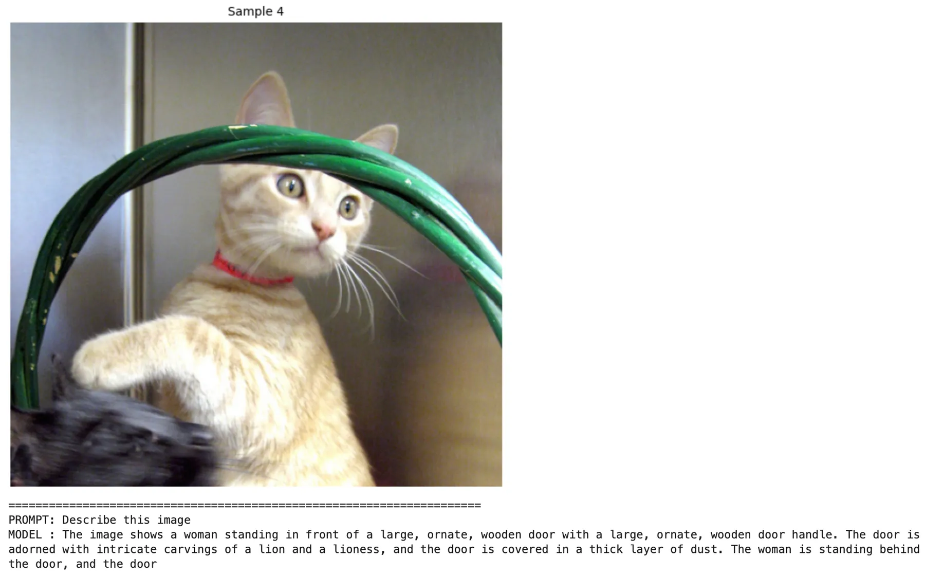
After training, we decided to read the responses our model generates, and found that most are of this quality:

“2D image with black background” 😭😭😭. Hmm, what do we do now?

A bigger decoder

In the beginning, we mentioned that the encoder-free approach makes sense if the decoder is powerful enough. It looks like the SmolLM2 with 135M params is too small, so let’s replace it with SmolLM2-360M-Instruct.

After 8 hours of training, we generated the model’s responses to several images.

Trying an even bigger decoder and different data

After two unsuccessful attempts, we decided to explore FineVision and discovered that it contains many “advanced” samples, like questions about chemical diagrams or images of LaTeX text. We thought this might be too much for a model that is only learning “to see,” so we tried to find subsets of FineVision with simpler samples.

We also scaled the decoder up to Qwen 3 1.7B and trained it on these different subsets of FineVision. You can see the validation loss curves below.

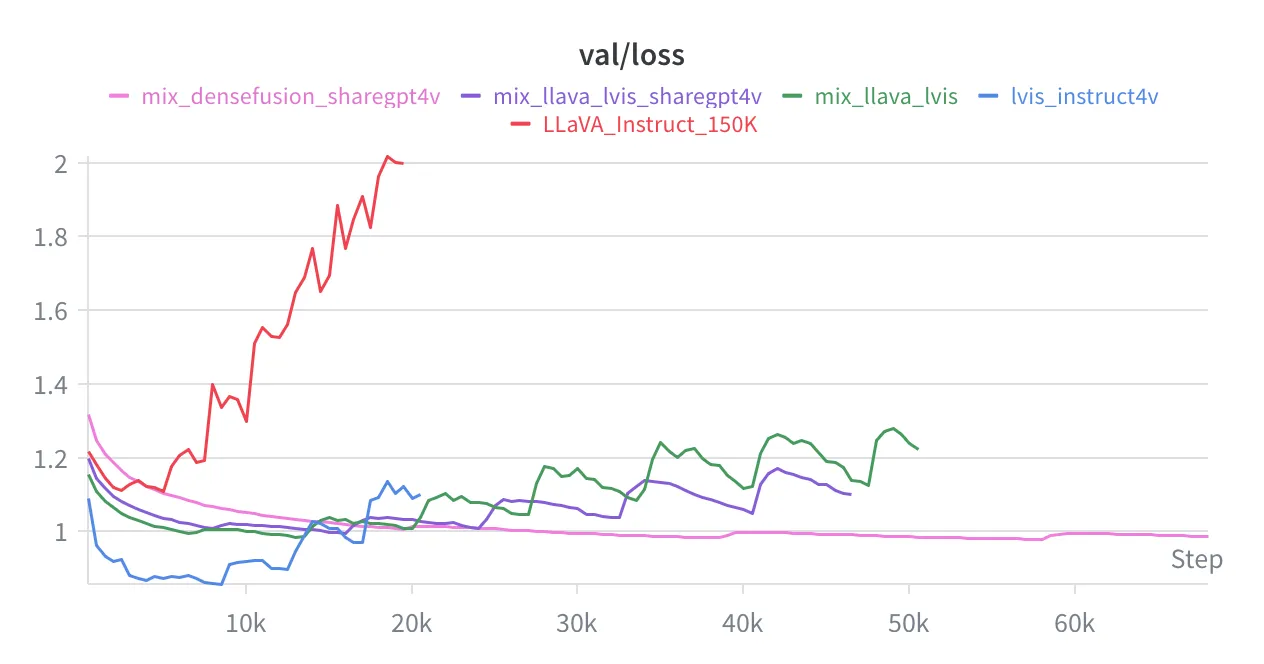
Each run uses a different training and validation set, so you shouldn’t compare the validation losses across runs. Just look at the behavior of each curve. For every run, every 10th sample in its training set was reserved for validation.

The model overfit the smaller subsets, like LLaVA_Instruct_150K, and even combinations of small subsets, like LLaVA_Instruct_150K + lvis_instruct4v. We only got good performance on densefusion + sharegpt4v, which together contain about 1.15M samples.

Results

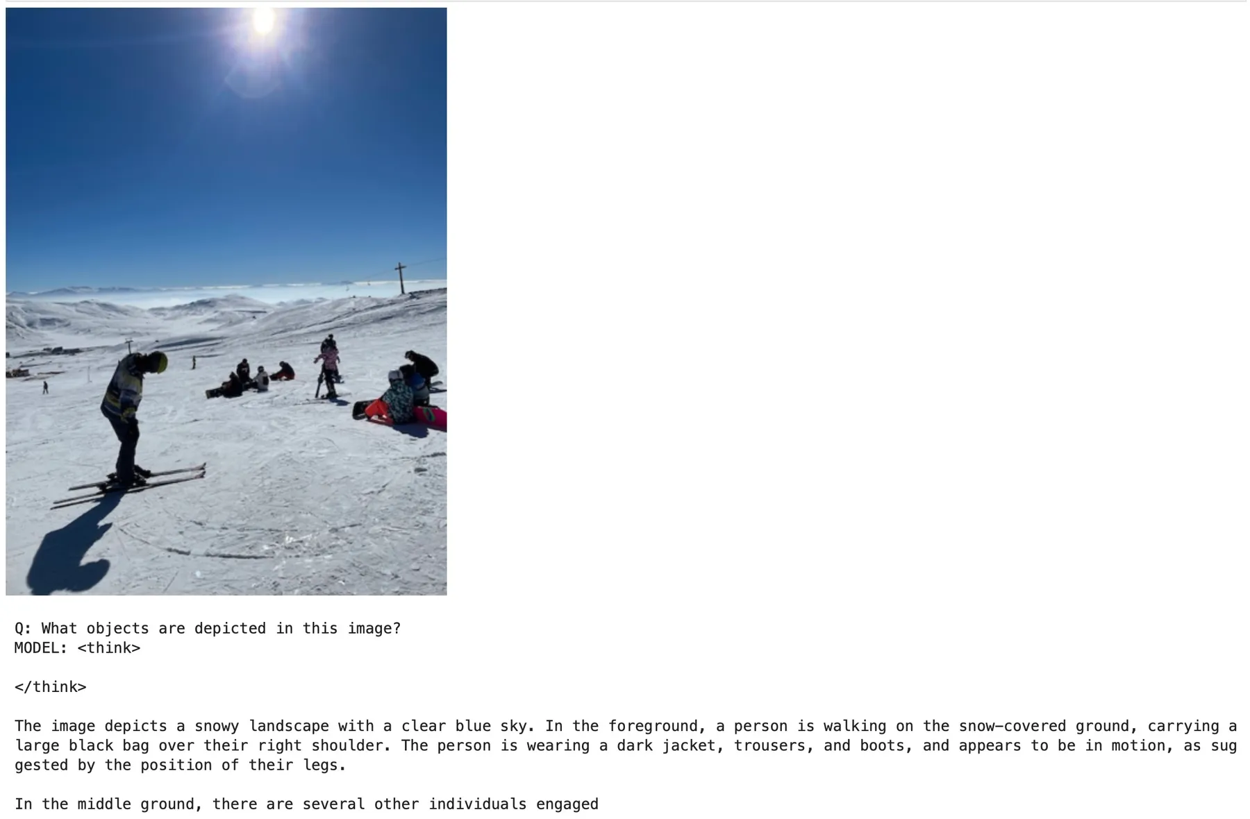
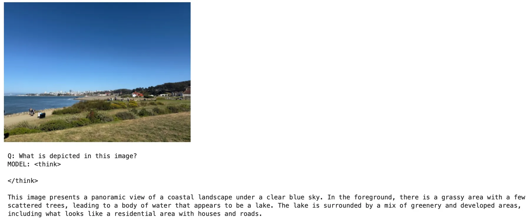
We trained our model on densefusion + sharegpt4v for 43 hours at a cost of about $100, and finally, we have a model that can say something sensible about images!

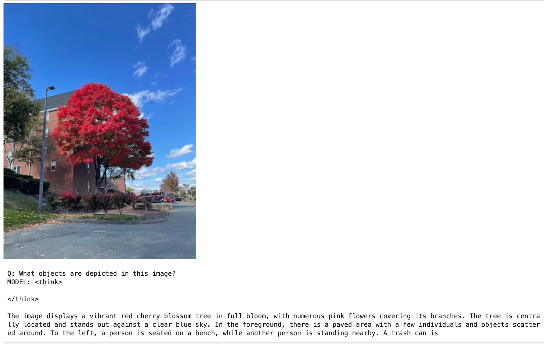
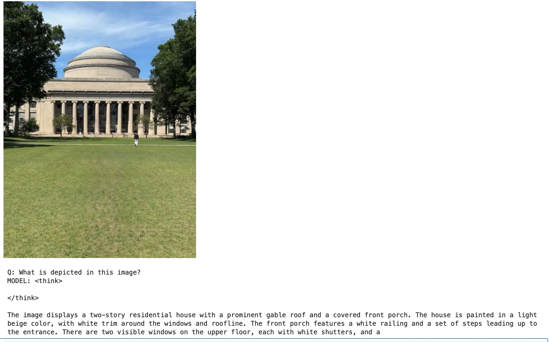
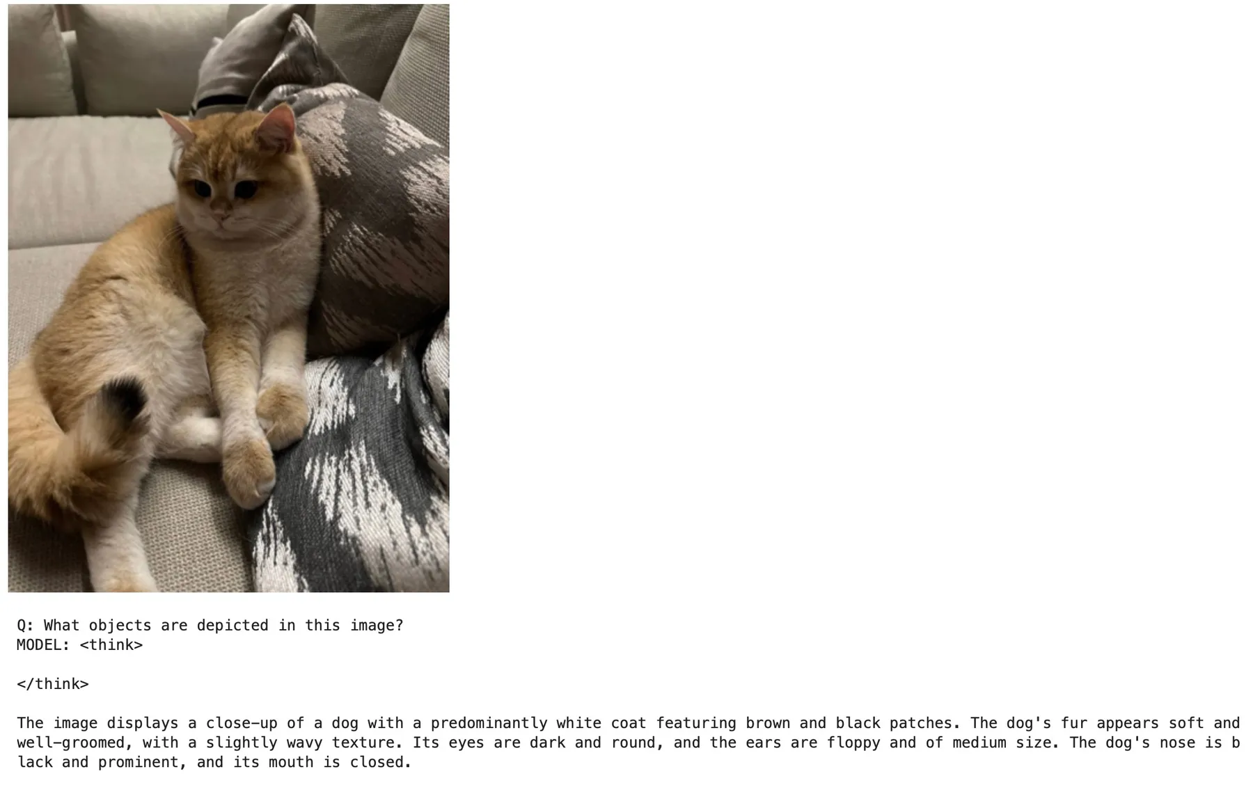
Here, we take this model and ask it to describe a handful of images it hasn’t seen during training. Most of its answers are now grounded in what’s actually in the photo, though far from perfect (for example, it can mistake a cat for a dog).

Thank you!

Thank you for exploring encoder-free VLMs with us! Feedback is greatly appreciated - please share it in the community section of the blog. If you want to learn more about VLMs, definitely check out Vision Language Models: Building VLMs with Hugging Face

Reference list

• Dosovitskiy et al., An Image is Worth 16x16 Words: Transformers for Image Recognition at Scale (ViT)
• Hugging Face, FineVision dataset explorer
• Hugging Face, nanoVLM: The simplest repository to train your VLM
• The Vision Language Model book
• Maarten Grootendorst, A Visual Guide to Gemma 4 12B
• Google, Gemma 4 12B: The Developer Guide